At the end of this tutorial, I have a bonus topic for you all which is quite rare but might come in pretty handy during the presentation. Spoiler Alert: It’s on Styling in Pandas.

Introducing Pandas

Pandas is a library that is built on top of NumPy. It offers several data structures that have a wide range of functionalities, which makes data analysis easier. We’ll talk about these Data Structures soon. It’s important that you know about NumPy, if you don’t you can learn about it here.

Apart from that, we’ll be doing data analysis over a real dataset. Yay!

What is a Series in Python Pandas?

Pandas contain Series which are the building blocks for the primary data structure in pandas i.e. DataFrames. Series are a 1-d array that has an index column and a label attached to it, along with other functionalities. You can think of a Series as a column in a spreadsheet. Let’s take a look at how you can create them.

Let’s start by importing pandas. Conventionally, we use pd as an alias for pandas.

import pandas as pd

Creating Series in Pandas

To start with Pandas, let’s take an example by creating a Series using the list. To do so, you just have to pass the list to pd.Series()

As you can in the above picture we created a list of numbers from 2 to 100 in reverse order and passed it pd.Series(), which created a series for it. The series output was 2 columns, the first one is an index column and the second one is the column that has the values of the list, along with the type and length of the series. One thing to note is that we didn’t require to print the series using print() to get an output.

It’s because in a jupyter cell the output of the object in the last line will be printed. Since in the last line of this cell we had our series object, its value was printed.

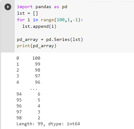
Now that we created a series using a list we can do it the same way for the NumPy array.

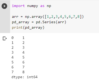
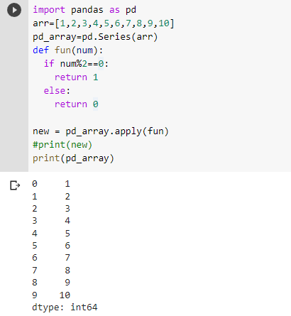
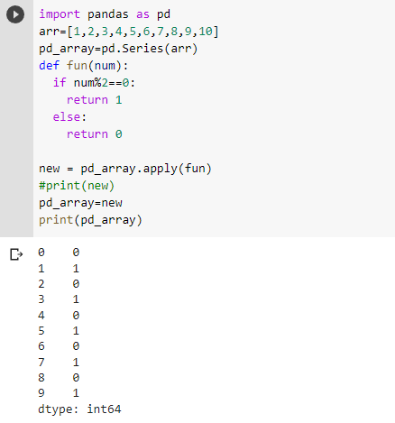
And as you can see we got a similar result. Now that we are familiar with how to create a series. Let’s take a look at how you can use one of its functionalities called apply(). What apply() does is that it takes in a function and applies it over each element and replaces the element with what the function returns. Let’s see how you can do it.

As you can see the even elements were replaced with 1 and odd elements were replaced with 0. We passed the function in apply() as an argument, the function returns 1 if the element is even and 0 if the element is odd. Therefore, even elements were replaced with 1, and odd elements were replaced with 0. But apply() doesn’t change the series itself, instead, it returns a transformed series leaving the original one the same.

But if you wanna keep the changes in the original series you can do so by assigning the transformed series to the original series object:-

We can also pass lambda functions as an argument and it’ll still work the same. If you don’t know about ternary operators you can read about them here.

DataFrames in Pandas in Python

If Pandas Series is a column of the spreadsheet, then DataFrames are the spreadsheet itself. DataFrame behaves the same way as an excel file. They have an index for corresponding rows and a label for each column.

Dataframes offer a long variety of functions that make data analysis easier, for example, summary statistics, column details, etc. We’ll take a look at how all this happens but first, let’s talk about CSV files if you are learning Pandas, you will need to work with CSV files for sure.

What is a CSV file?

CSV stands for Comma Separated Values. In a CSV file, the elements are separated by a ‘,’. Pandas actually have a function read_csv() which you can use to easily load the contents of a CSV file into a data frame. Let’s see how.

Pandas DataFrame Operations

Loading CSV file into a DataFrame

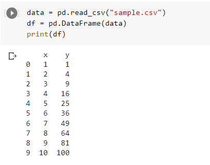
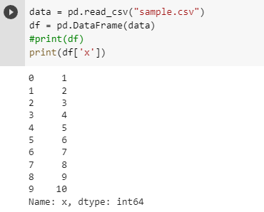
As you can see there are 2 columns. 1st column has the name x and 2nd column has the name y. In the data frame, you can get the values stored in each column individually by calling the columns by their name themselves.

Now one last thing, earlier I said that if a series is a column then the data frame is a spreadsheet. Does that mean that DataFrames are a collection of series? Short answer, Yes. Every single column in DataFrame is a Series.

Adding a column in DataFrame in Python Pandas

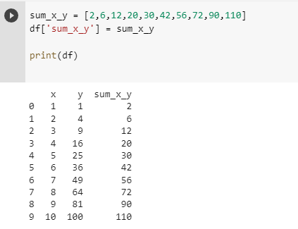
Adding a column in Dataframe is as easy as declaring a variable. Just call the name of the new column via the data frame and assign it a value. You can also create new columns that’ll have the values of the results of operation between the 2 columns. Let’s create a column ‘sum_x_y’ that has values obtained by adding each element of column x with the corresponding value in column y.

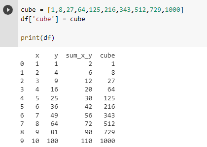
Let’s add another column that’ll have a cube of elements in column x.

Deleting a Column in Pandas DataFrame

Deleting a column in a data frame can be done using the del keyword or drop() function. Let’s see how you can delete a row using del.

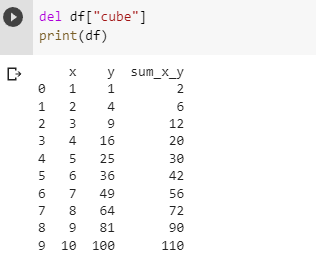
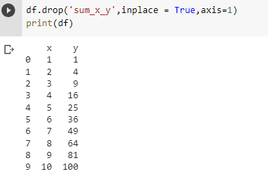
As you can see the deletion was inplace and changes were reflected in the original data frame. Now let’s see how you can delete a column using drop().

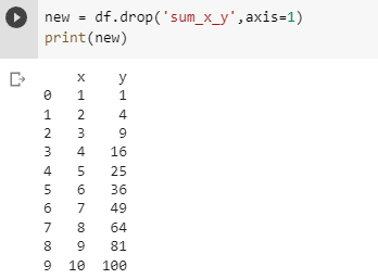
As you might have figured out drop() doesn’t do the changes in the data frame itself, rather it returns a transformed data frame but doesn’t change the original data frame. We used axis = 1 to tell that the element to be deleted is across the column.

In order to do the changes in the original data frame itself, you can pass another argument inplace = True. You can also delete multiple columns at the same time bypassing the list of columns.

Selecting Data based on a Condition

Like np array’s boolean indexing you can select rows in a data frame based on a condition.

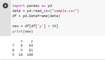
And like that, you can select rows based on a condition. Applying relational operators over a data frame created a boolean series that contains a bool value signifying whether the rows fulfill the condition or not. Passing it to the data frame will return a data frame with rows that follow that condition.

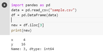
iloc method

iloc method can be used for slicing data frames. Slicing works the same way as it did in NumPy.

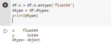
Changing dtype and names of a columns

Let’s start by creating our data frame. Now that we have our data frame. Let’s check the dtype of columns.

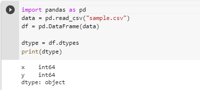
As seen the dtype of the column is int. We can change it to string or any other datatype using astype() method. Let’s see how.

Saving a DataFrame as CSV File

You can save Pandas dataframes as CSV files to using the method to_csv().

demo.to_csv('demo.csv')

We can actually convert dataframes to various other formal using to_numpy(), to_list() etc.

Data analysis using Python Pandas: A Practical Example

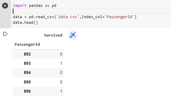
Now let’s get our hands dirty with some real-life data analysis to dive deep into the world of Pandas. For that, I’ll be using the Titanic Dataset. Let’s start by loading our data.

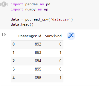
So as you can see we loaded our data using read_csv() and displayed the first 10 rows by using head(), the number passed as an argument in the head() is the number of rows that will be printed from the top. The default number of rows for the head() is 5.

In order to look at the n rows from the bottom, you can use the tail() method.

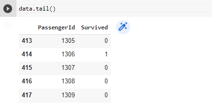
And as you can see it shows that the last 5 rows were displayed and one more thing to notice is the first column, marked with an arrow, with bolded no. this column is called the index column and you can customize this too.

Won’t it be more appropriate for our PassengerID to be the index column? Let’s try making it the index column.

Creating Custom Index Column

Method 1: Using the set_index method

We can change the index column by passing the name of the new index column as an argument to the set_index() method.

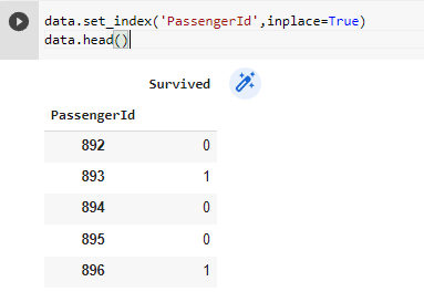
And you can actually create multiple index columns.

Method 2: By Passing column name as an argument

Apart from the method above, you can also pass the name of columns you wanna make an index in form of a list to the index_col argument in the function pd.read_csv().

Data Exploration

Now that we know how to load the data we should understand the data. Understanding what the data is and what it interprets plays an important role in data science and before preprocessing the dataset one must understand the dataset. And that’s what data exploration is all about.

Shape of Data

Before starting any sort of exploration or cleaning it is better to understand the basic layout of data and by that I mean no. of rows and columns in the dataset. Let’s see how you can find it and how to interpret it.

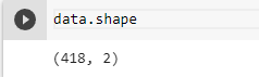
We received a tuple with 2 values. The first value is the no. of rows and the second value is the no. of columns. So as seen in the image the no. of entries is 891 and the no. of features is 12.

Fetching Column Info

Now that we know the basic layout of the data let’s understand it in a bit more detail. So the next thing to do is to get a basic idea about the features in your dataset like if any column has any missing value and the dtype of the features. To get that we use the info() method.

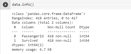
info() method is used to get the summary of the dataframe. Let’s understand its output with the above image as an example:-

• Total Entry and Index Range(Blue Arrow): Tells the no. of entries in the data set along with the first entry of the index column in this case 0 and the last entry of the index column in this case 1.
• Feature Name: Among the 4 rows, the 1st column is Serial No. columns and the 2nd column is the column that contains the names of our features in the dataset.
• No. of Non-Null Rows(Dotted Rectangle): This column contains the total no. of non-null entries in the corresponding feature. If this value is the same as the total no. of rows then there are no null values in the column else there are missing values.
• Dtype of the column(Purple Box): This column contains the dtype of the corresponding feature. You can go through this column and check if any column is of unsuitable dtype and change it to the correct one if necessary.
• Red Arrow: Summary about no. of columns having the corresponding type. This one has 2 float features, 5 int features, and 5 object features.

Fetching the Descriptive Statistics of the Dataset

Pandas provide us with mean(), median(), quartile(), etc. methods using which we can fetch the statistics of a dataset. But doing it for each column can be a tedious task. This is where the describe() method comes to the rescue.

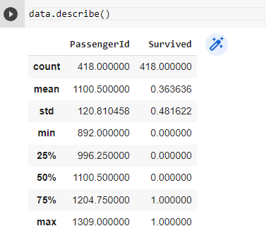
This method provided us with the statistics for the numerical columns but we can also check statistics for categorical columns by passing argument include = ‘all’.

Let’s understand the output:-

• count: No. of non-null values.
• unique: No. of unique classes in a categorical column.
• top: Category with max frequency.
• freq: Frequency of the most frequent class.
• mean: Mean of the corresponding column.
• std: Standard Deviation of the corresponding column.
• min: Minimum Value in the corresponding column.
• 25%,50%,75%: 1st,2nd(median),3rd Quartile of the corresponding column.
• max: Maximum Value in the corresponding column.

No. of Classes and its frequency in a Categorical Column

When dealing with categorical columns you might want to know the classes it has and their frequency. For that, we can use:-

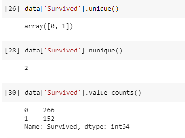
• unique(): This method returns all the classes that the column has including nan.
• nunique(): This method returns the no. of classes that column has excluding nan.
• value_counts(): This method returns the classes and their frequency in that column, excluding nan.

Data Cleaning in Python Using Pandas

Removing Useless Columns

Understanding which column is useful and which one isn’t is an important task that can be done in many ways. One of them is intuition. For example, in this dataset, we have to predict based on data if someone survived or not.

Handling Missing Values in Pandas

Missing Values, also known as NaN values, is the result of an entry in a row that doesn’t exist. NaN stands for Not a Number. So how to find how many NaN or null values a column has?

It’s simple we find which entries are null and assign a bool to it and then find the sum of that bool matrix along with the columns. That no. will be the no. of Null Values.

As we can see Age has 177 NaN values and Embarked has 2 NaN values. Usually, ML models can fetch an error if trained on missing values, hence we usually tackle them by:-

Dropping rows with NaN Values:-

One way to tackle NaN values is to remove the rows having NaN values from the dataset. If the column has a lot of NaN values we usually won’t take this approach.

As you can see now the Embarked column now has no NaN values. Alternatively, you can use dropna() method on the column from which we wanna remove those entries.

Replacing NaN Values with another Value

Age has 177 NaN values, so unlike Embarked, we can’t delete entries since it’ll result in the loss of a lot of information.

Another way to tackle NaN values is to replace NaN with something else like mean, median, mode, etc. What to replace them with is a different topic but for now, let’s replace it with mean age using fillna() method.

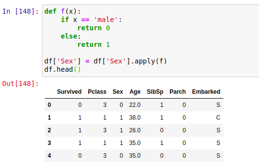
Handling String Values in Python Pandas

Usually, ML models need data to be strictly numerical thus any sort of string data can cause an error. Therefore we need to handle this by converting string data to numerical data. For this, we’ll create a function that’ll map the classes to an integer and use apply() to apply that function to all the elements.

We have 2 columns with string values i.e. Embarked and Sex. Sex has 2 classes [‘male’,’female’] who we’ll replace with [0,1] respectively.

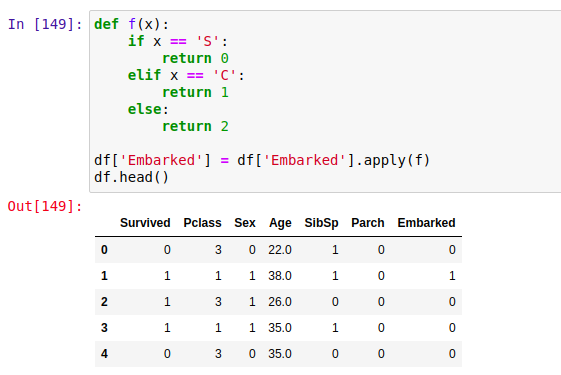
Embarked has 3 classes [‘S’,’C’,’Q’] who we’ll replace with [0,1,2] respectively.

Hooray! You just did your first data preprocessing task. Now There are many more things that are to be done and we’ll go into details about them but for now, this dataset is good enough to train a model.

Styling in Pandas

Time for the promised bonus topic. Now let’s suppose you wanna show the Age column in the format x year you can do that using format() method and specifying the display format for the corresponding column.

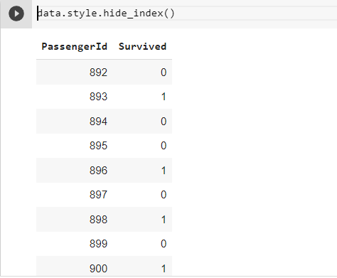
If you don’t wanna show the index column you can use hide_index().

There many interesting things you can do with styling but that’s an article for another day. The aim was to introduce you to the concept of Styling in Pandas. Hopefully, you liked it and enjoyed it.